A few optimisers

Notation§

We assume the standard neural network training setup.

Our network is parameterised by a high-dimensional vector, which we will write as $\theta$.

We are trying to minimise some loss function, which takes both the parameters of the network and a dataset. We will call the dataset $X$, and we will call batches sampled from the dataset $x$.

We will express “the loss on batch $x$ given parameters $\theta$” as $\ell (\theta, x)$.

The gradient (direction of steepest ascent) of the aforementioned loss is written $\nabla \ell (\theta, x)$.

We will express our optimisers in terms of update rules, declaring the value of a quantity in terms of quantities obtained in an earlier step or in a prior update rule. This will look like this:

$$v_{t+1} = 2v_t$$

For a sequence of $v$s that doubles at each time-step.

Hyperparameters§

Optimisers are often parameterised by constants, called hyperparameters.

The most important hyperparameter is the learning rate, written with the symbol $\alpha$. Optimisers can vary their hyperparameters over the course of their execution – this is called hyperparameter scheduling.

Scheduling the learning rate in particular is extremely important for good performance.

Initialisation§

Writing optimisers in terms of update rules ignores the initial state of the variables at $t = 0$. There are different ways to initialise $\theta$. It is generally safe and effective to pick He initialisation.

Gradient Descent§

Gradient descent has a single hyperparameter, the learning rate $\alpha$.

The rule is to take a small step in the negative direction of the gradient at each time-step:

$$\theta_{t+1} = \theta_t - \alpha_t \nabla \ell (\theta_t, X)$$

Stochastic Gradient Descent§

Because computing the loss over the whole dataset is slow, we can instead compute it over a sampled subset of the dataset:

$$\theta_{t+1} = \theta_t - \alpha_t \nabla \ell (\theta_t, x_t)$$

This is Stochastic Gradient Descent (SGD).

This introduces a new hyperparameter, the batch size. All optimisers from here on in will have this hyperparameter, and I shan’t make further comment on it.

Momentum§

An issue with SGD is that it introduces noise. A well-performing addition to SGD is to keep an exponential moving average (EMA) of the gradients, and to update the parameters in the direction of the average, rather than the gradients. This has the effect of smoothing out oscillating noise in favour of coherent directions in parameter-space.

$$\begin{align*} m_{t+1} &= \beta_1 m_t + (1 - \beta_1) \nabla \ell (\theta_t, x_t) \\ \theta_{t+1} &= \theta_t - \alpha_t m_{t+1} \end{align*}$$

This introduces a new hyperparameter, $\beta_1$, which is usually well-set at $0.9$ or so. Like $\alpha$, $\beta_1$ can be scheduled, but this is far rarer for these parameters, so here and onward I have omitted the $t$ subscript.

RMSProp§

RMSProp is similar to Momentum, but it maintains an EMA of the squaredWhat does it mean to square a gradient? In this case, we are thinking of gradients as simply being big lists of numbers in one-to-one correspondence with the network’s parameters, that say whether a parameter should increase or decrease, and by how much. When we speak of “squaring” the gradient, we mean squaring each number in this list. gradient instead of the gradient itself.

This running average, called $v$, is used to obtain $\sqrt{v}$, an estimate of the root-mean-square of the recent gradients.

RMSProp scales the gradient by the inverse of this value, shrinking components of the gradient that have been recently large, and magnifying recently-small gradients.

$$\begin{align*} v_{t+1} &= \beta_2 v_t + (1 - \beta_2) \nabla \ell (\theta_t, x_t)^2 \\ \theta_{t+1} &= \theta_t - \alpha_t \frac{1}{\sqrt{v_{t+1}} + \epsilon} \nabla \ell (\theta_t, x_t) \end{align*}$$

$0.999$ is a good value for $\beta_2$.

Adam§

Adam is a combination of Momentum and RMSProp. It keeps EMAs of both the gradient and its square, updating parameters in the direction of the EMA of the gradients, scaled by the root of the EMA of the squared gradients. We call the gradient EMA parameter $\beta_1$, and the squared gradient EMA parameter $\beta_2$.

$$\begin{align*} m_{t+1} &= \beta_1 m_t + (1 - \beta_1) \nabla \ell (\theta_t, x_t) \\ v_{t+1} &= \beta_2 v_t + (1 - \beta_2) \nabla \ell (\theta_t, x_t)^2 \\ \theta_{t+1} &= \theta_t - \alpha_t \frac{1}{\sqrt{v_{t+1}} + \epsilon} m_{t+1} \end{align*}$$

Adam is an extremely well-performing optimiser, and in many cases is difficult-to-impossible to improve upon.

Intermission: Learning Rate Schedules§

All of the aforementioned algorithms require their learning rates to be changed over the course of execution for good performance.

There are many extant approaches to learning rate scheduling.

Step

Linear

Cosine

Exponential

Warmup-Stable-Decay

One-Cycle

Cosine Restarts

Inverse Square Root

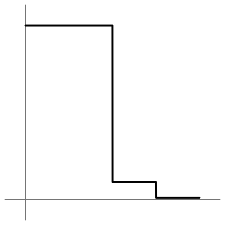
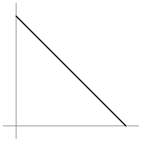
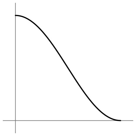
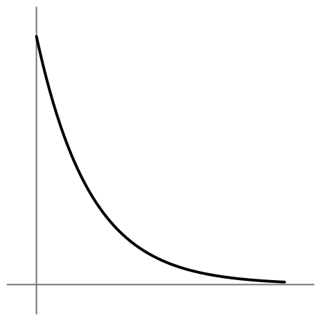
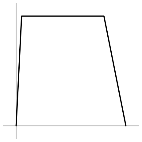
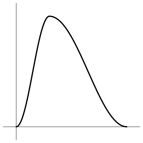
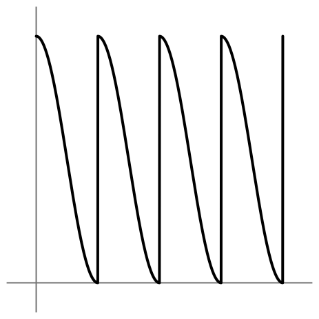
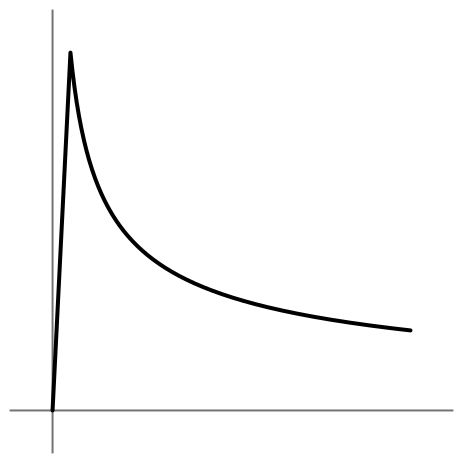
If in doubt as to which you should use, I recommend linear.

Schedule-Free Learning§

Somewhat more than two years later, I have learned to read. In particular, I have read Aaron Defazio et al’s The Road Less Scheduled.

The summary (as I understand it) is this – first, learning rate schedules are theoretically unjustified. Optimisation theory states that for optimal performance, $\alpha$ ought to be constant over the course of training.

Not only that, but theory also recommends taking the average of the $\theta$ iterates $\theta_0$ to $\theta_T$ as your trained parameters, rather than the final value, as practitioners do.

Neither constant learning rates nor uniform iterate averaging are anything other than garbage when actually attempted in practice.

The interesting claim that this paper makes is that learning rate schedules effectively implement iterate averaging in a manner that conforms to theory while also working in practice. In particular, a linear learning rate decay corresponds to an equal-weighted average of iterates.

The authors then ask:

They say yes, and call this Schedule-Free Learning.

Schedule-Free SGD§

Recall normal SGD:

$$\theta_{t+1} = \theta_t - \alpha_t \nabla \ell (\theta_t, x_t)$$

Each step, we move $\theta$ in the direction of the negative gradient.

Now, consider if we instead kept a running average of all previous iterates:

$$c_{t+1} = \frac{1}{t+1} \\ \begin{align*} \theta_{t+1} &= \theta_t - \alpha_t \nabla \ell (\theta_t, x_t) \\ \mathtt{avg}_{t+1} &= (1-c_{t+1}) \mathtt{avg}_t + c_{t+1} \theta_{t+1} \end{align*}$$

As mentioned before, this doesn’t work at all – $\mathtt{avg}$ is a terrible parameterisation for the network in practice.

Now, consider this alternative procedure:

$$c_{t+1} = \frac{1}{t+1} \\ \begin{align*} y_t &= (1 - \beta) z_t + \beta\ \theta_t \\ z_{t+1} &= z_t - \alpha \nabla \ell (y_t, x_t) \\ \theta_{t+1} &= (1-c_{t+1}) \theta_t + c_{t+1} z_{t+1} \end{align*}$$

Several things have occurred at once.

First, note that I have suggestively removed the $t$ subscript from $\alpha$.

Second, note that $\theta$, our network parameters, is now an equal-weighted average of a quantity, called $z$, which I will refer to as the fast weights. $z$ is (almost) a normal SGD iterate.

Third, we have introduced a new sequence, $y$, that is an interpolation between the fast weights and our real parameters.

Lastly, note that we are updating the fast weights $z$ using a gradient computed at $y$!

I have shown you the update rule for the algorithm that Defazio et al call Schedule-Free SGD, and they find that it performs as well or better than SGD with a well-tuned learning rate schedule. Look how good these curves look:

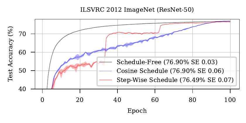
There are two main features of Schedule-Free that make it so attractive. First, that it sweeps out the entire Pareto frontier of training-time / loss, providing the best possible iterate anytime. Second, one does not have to experiment with schedules, making it easier to get the ideal performance with reduced work tuning hyperparameters.

Schedule-Free can wrap any optimiser, and the authors also provide a reference implementation of Schedule-Free AdamW, which performs even better.

Making it work§

I implemented Schedule-Free AdamW in bullet, the state-of-the-art trainer for chess engine NNUEs. I’ve been having promising results in some initial experiments, and have been beating Ranger in small experiments:

These curves still look a bit weird, and I’m not confident I’ve implemented everything correctly, and I’m not sure if or how Schedule-Free can cope with non-stationary objectives like the one I used in Stage 1, but I’m nevertheless excited and hopeful about this method.

Results§

※ This section was added after the writing of the initial note.

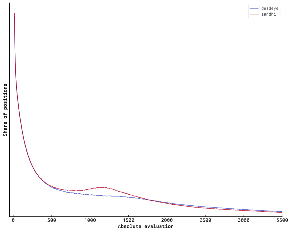
A full run with Schedule-Free AdamW was completed, getting lower final loss than the Ranger baseline:

The shape of this curve is very similar to the test curves.

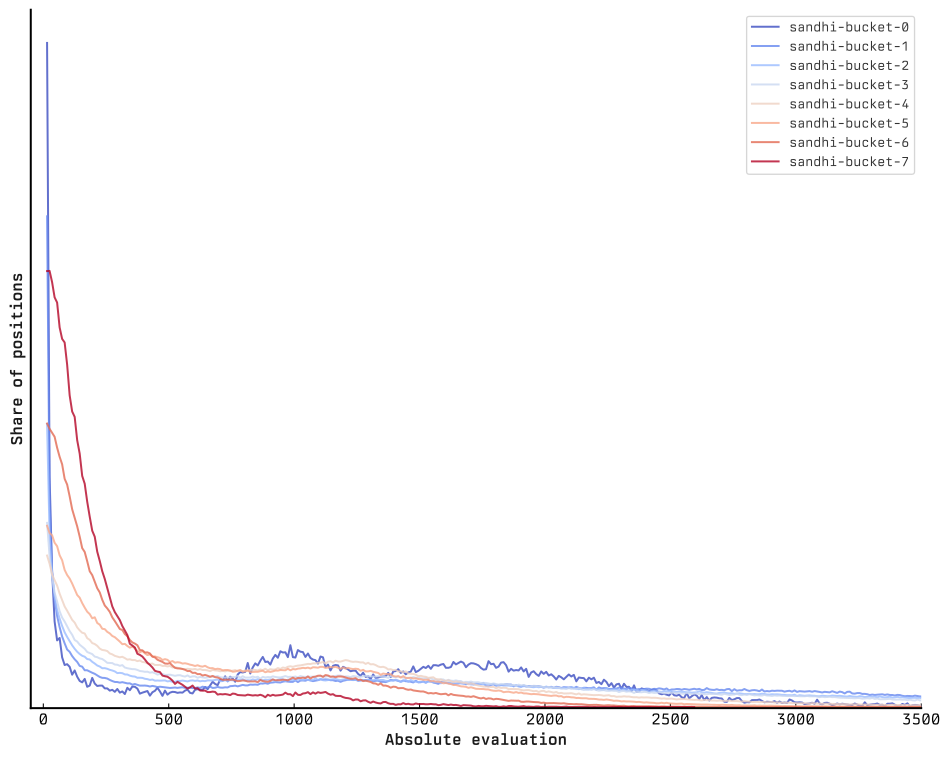
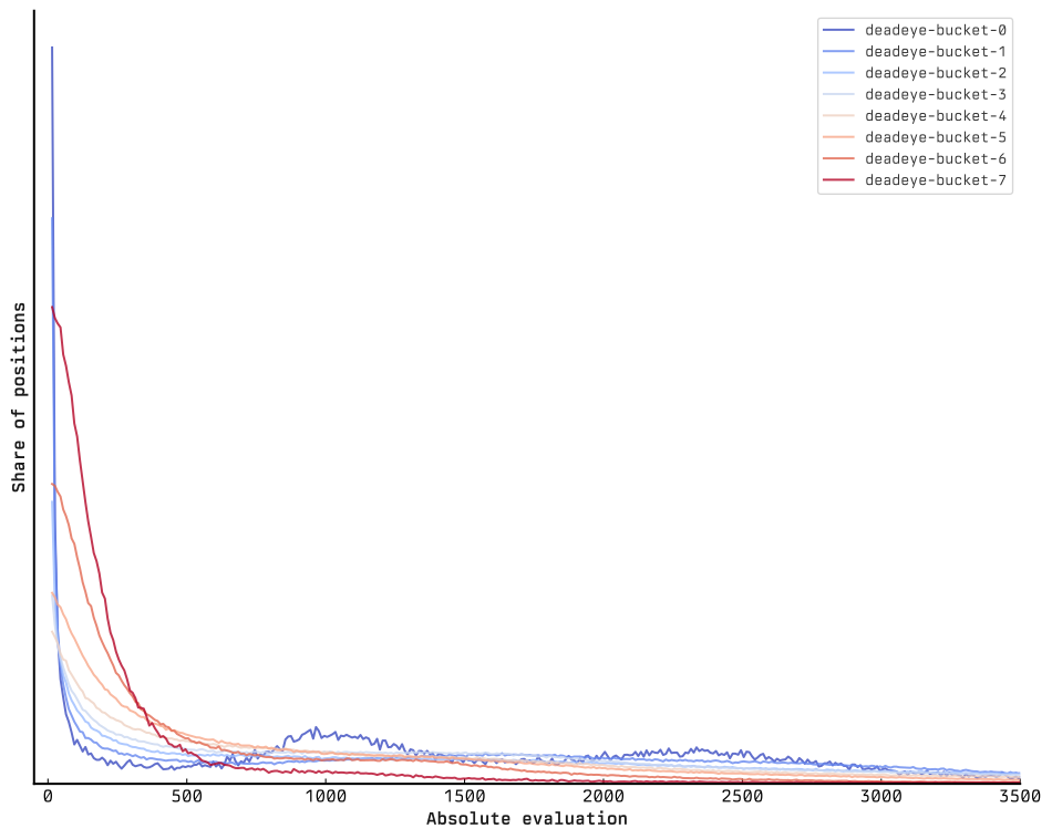
The evaluation scale of this new network is somewhat different:

Unfortunately, this network did not prove stronger.

  LLR −3.13 (−2.94LO +2.94HI BOUNDS for +0.00LO +3.00HI ELO)
  ELO −4.55 ± 3.48 (−8.03LO −1.07HI)
 CONF 25 KNODE (1 THREAD 16 MB CACHE)
GAMES 13978 (3983W28.5% 5829D41.7% 4166L29.8%)
PENTA 213+2 1600+1 3193+0 1757−1 226−2

  LLR −2.96 (−2.94LO +2.94HI BOUNDS for +0.00LO +3.00HI ELO)
  ELO −5.12 ± 3.43 (−8.55LO −1.69HI)
 CONF 8+0.08 SEC (1 THREAD 16 MB CACHE)
GAMES 10392 (2555W24.6% 5129D49.4% 2708L26.1%)
PENTA 31+2 1165+1 2657+0 1306−1 37−2

✦✦✦